Equations

One of the most egregious communication flaws by students of mathematics is an inappropriate use of the = symbol. Often, students use it as a way of saying, I've worked through this little bit of a calculation and found this answer, and then just keep on working. Also, it is often used or interpreted as a statement of assignment, when it should not be.

Before we discuss the proper use of =, we need to make a distinction between a numerical value and a logical value. A numerical value is something that represents an actual number. Constants, variables, and expressions are all examples of mathematical objects that have numerical values, such as 5, $\pi$, $x$, or $x^2-3x$. A logical value is either true or false. Statements have logical values, such as It is raining, 4 is a prime number, or Harrisonburg is the capital of Virginia. Notice that a statement does not have to be true to be logical. It merely must be capable of determining whether it is true.

An = sign is used to create a logical statement that two expressions have the same numerical value. This type of statement is called an equation. An equation can be (1) always true, (2) sometimes true, or (3) always false. Each of the following are examples of equations: \[\begin{align*} 1+1 &= 3 \\ 2(x+3) &= 2x+6 \\ 3x+1 &= 2x-5 \end{align*} \] Could you decide whether each equation is always true, sometimes true or never true?

Why Equations?

Recall that an expression typically is a model for some physically measured quantity. It is often of interest to form an equation to represent the condition that two comparable physical measurements have the same value. The equation then is formed by stating that the two expressions have the same value. The mathematical task is then to identify a strategy that will allow us to determine which values of the independent variable(s) make the statement true.

The process of following a strategy to identify which values of the independent variables will make the equation true is called solving the equation. One possibility is that the equation will always be true, in which case the two measurements are curiously actually measuring the same thing, perhaps in different ways. It is also possible that the equation will never be true, in which case the two measured quantities must always be different. Or it is possible that the equation will be true only for particular values of the independent variable. Mathematicians call the collection of possibilities that make the equation true the solution set and each particular value is called a solution.

Right now, we will focus only on the ideas of an equation and its solutions. We will return to strategies for solving equations after we understand what we are trying to find.

Example: You have a pre-paid cell phone account that charges $0.15 per text message. Your current balance on the account is $24.75. If you don't make any calls, how many text messages can you make?

It is entirely possible to work through this problem without ever introducing the idea of an equation. However, it is our goal to use the example to reinforce the ideas of equations.

We start by identifying the variables. You get to choose how many text messages you send. So this is one variable — let us use $T$ to count the number of text messages. The cost resulting from your text messages is another variable, and it is determined from $T$ — let us use $C$ to represent the cost of your text messages. Mathematically, we can now identify the equation we seek to solve. We want to solve the equation $C = 24.75$ for the variable $T$.

However, unless we have a model for the cost as a function of the number of messages, we are not yet ready to proceed. The cost $0.15 is called a unit-cost so that the total cost is the unit cost times the number of units, \[ C = 0.15 T. \] This is an example of a proportional model, where the unit-cost is the proportionality constant (the rate). Using the model, the equation we wish to solve is \[ 0.15 T = 24.75. \] You likely know how to solve this particular equation, dividing both sides by 0.15, to obtain $T=165$. That is, sending 165 text messages will result in charges to your account $C$ that exactly depletes your existing balance of $24.75.

Example: In economics, it is common to consider a balance between supply and demand. Consider a commodity, for example, an ultra-high-grade chocolate. If the price of chocolate is low, demand will be high meaning that people will buy a lot of chocolate. But if the price is raised, then the amount of chocolate that is purchased will decrease. On the other hand, the chocolate companies are interested in higher prices. If the price is low, there is not much interest to supply the chocolate. If the price is raised, the companies have greater interest in supplying more chocolate.

Let $p$ represent the price per pound for chocolate, let $D$ represent the number of tons that the consumers would demand at the price $p$, and let $S$ represent the number of tons that the companies would supply at the price $p$. Real supply–demand curves are more complex, but suppose that we can use linear models such as the following: \[ \begin{align*} S &= 20p-100 \\ D &= 100-5p \end{align*} \] Notice that our models, themselves, were expressed as equations. That is, we had two dependent variables, $S$, which was the measurable outcome, and the expression, $20p$, and the equation states these are equal, with an implicit assumption that this is always true (or at least true for all relevant values). The supply–demand balance point is where the consumers purchase everything produced, namely where supply and demand are equal, $S=D$. This leads to the equation that we would actually attempt to solve, \[20p-100 = 100-5p.\]

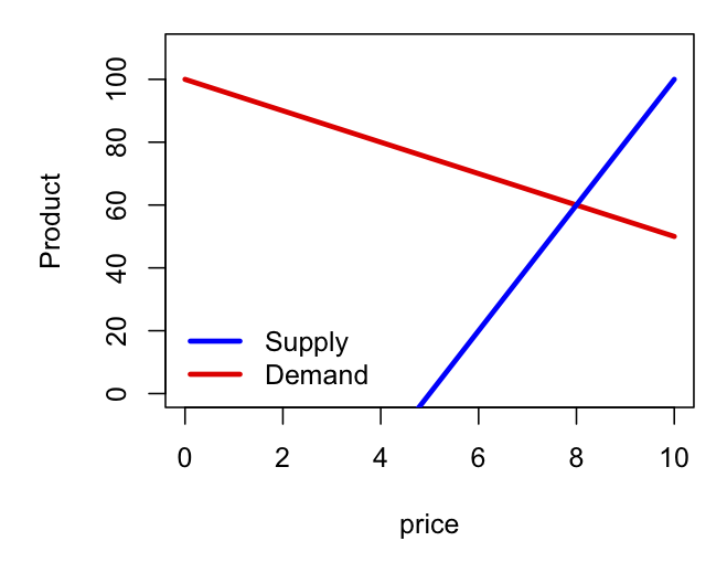A graphical representation of these supply and demand functions of the price is shown to the right. The solution corresponds to the price where the two functions yield the same value. If the price is too high, the supply is greater than the demand, resulting in a glut of supply and not enough demand. If the price is too low, the demand exceeds the supply. But at the solution $p=8$, there is a perfect balance with demand exactly matching supply.

In summary, from the perspective of models, the most common reason to use an equation is to find the value or values of an independent variable so that either a dependent variable attains a particular value of interest or that two different dependent variables attain the same unspecified value.

Identities

Mathematically, there is another type of equation that is particularly important called an identity. An identity is an equation involving two different expressions that always have the same value as a consequence of algebraic rules. Identities are often used in substitution, where one expression within a formula is replaced by its equal. In a sense, all of algebra is based on the collection of valid identities. Most of the equations given in Section 0.2 of the textbook, Equations, are actually identities, while only a few steps are related to solving equations as we have been discussing.

The most important identities are based on the fundamental properties of addition and multiplication.

Subtraction and division are really just addition and multiplication in disguise. Subtraction $a-b$ corresponds to addition using an additive inverse, \[a-b = a+-b.\] Division $a / b$ corresponds to multiplication using a multiplicative inverse, \[\frac{a}{b} = a \cdot \div b,\] which of course requires that $b \ne 0$ for the inverse to exist. Two additional identities are often necessary, \[ \begin{gather*} -(a+b) = -a + -b, \\ \div(a \cdot b) = \div a \cdot \div b. \end{gather*} \] The first of these states that the additive inverse of a sum is the sum of the additive inverses; the second states that the multiplicative inverse of a product is the product of the multiplicative inverses.