Inequalities

Example: Interpret the inequalities \(x^2 < x+2\) and \(x^2 > x+2\) by using the graphs \(y=x^2\) and \(y=x+2\).

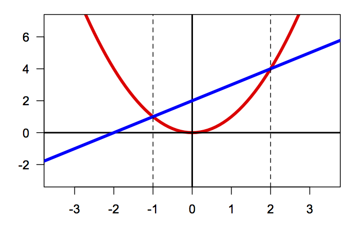
The graph shows \(y=x^2\) in red and \(y=x+2\) in blue. Two vertical dashed lines are also shown where the two graphs cross, that is at the solutions to \(x^2=x+2\). For \(x<-1\), we see that the red graph is above the blue graph, \(x^2 > x+2\). For \(x>-1\) and \(x<2\), the red graph is lower, \(x^2 < x+2\). For \(x>2\), we have \(x^2 > x+2\) since the red graph is once again above the blue graph.

Solution sets to inequalities are usually expressed using interval notation. This is discussed in Section 0.1 of the textbook. The inequality \(x^2 < x+2\) is true when \(x>-1\) and \(x<2\), which is written in set notation as \[ \{x: x^2 < x+2\} = \{x : -1 < x < 2\} = (-1,2). \] The inequality \(x^2 > x+2\) has a solution set the involves two disjoint intervals, \(x<-1\) as well as \(x>2\). Logically, a particular value \(x\) can only satisfy one of the inequalities, so we say \(x<-1\) or \(x>2\). In set notation, the solution set is written \[ \{x : x^2 > x+2\} = \{x : x < -1 \hbox{ or } x>2\} = (-\infty,-1) \cup (2,\infty). \]

Example: Interpret the inequalities \(x^2 < x+2\) and \(x^2 > x+2\) by using the graph of \(y=x^2 - (x+2)\).

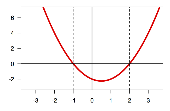
This inequality is the same as for the previous example. If we view the difference \(x^2-(x+2)\) as \(A-B\), then we view the graph as how much we need to change to go from \(y=x+2\) to reach \(y=x^2\). In fact, you should compare the graph of the difference shown here with the graphs of the two expressions in the previous example. Can you see how the graph \(y=x^2\) is above \(y=x+2\) whenever the graph of the difference is positive (above the axis)?

The difference is positive for the values \(x\) with \(x<-1\) and for the values \(x\) with \(x>2\). This allows us to interpret the solution set \[ \{x : x^2 > x+2\} = \{x : x < -1 \hbox{ or } x>2\} = (-\infty,-1) \cup (2,\infty). \] On the other hand, the difference is negative for the values \(x\) with \(x>-1\) and \(x<2\), giving us the solution set \[ \{x: x^2 < x+2\} = \{x : -1 < x < 2\} = (-1,2). \]

Because the comparison for the difference is with zero, we can identify the two points where the difference equals zero using factoring. The difference is \(x^2-x-2\) which can be factored \(x^2-x-2=(x-2)(x+1)\). Solving the equation \(x^2-x-2=0\) is then transformed into finding those values \(x\) for which \(x-2=0\) or \(x+1=0\), which gives the two solutions \(x=2\) and \(x=-1\).

Example: Express \(\{x : |x-3|<2\}\) using interval notation.

The inequality \(|x-3|<2\) is an absolute value inequality, so it can be interpreted in terms of distance. There are multiple perspectives to the inequality, all of which give the same result.

The most direct approach is to do pattern matching with \(|A-B| < \delta\) and recognize that the inequality \(|x-3|<2\) has the distance interpretation that the distance between \(x\) and \(3\) is less than 2 (alternatively read as at most 2). Since 3 is a definite number, we can mark it on the number line and travel a distance 2 in both directions to reach the numbers 1 and 5.

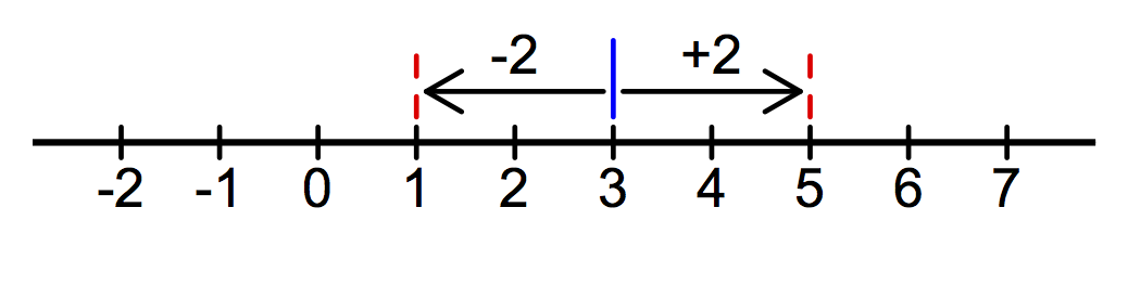
The numbers whose distance from 3 is less than 2 are those that are between 1 and 5. \[ \{x : |x-3| < 2\} = \{x : 1 < x < 5\} = (1,5). \]

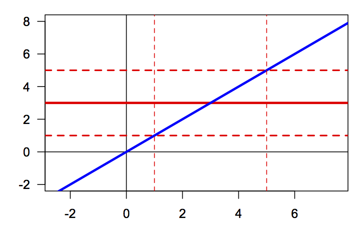
A second approach is to think of \(x-3\) as an expression that we can graph. The inequality \(|x-3| < 2\) can also be interpreted as saying that this expression is at most 2 units away from 0, which is the horizontal axis. So a graphical interpretation of this inequality would show the graph \(y=x-3\) along with horizontal lines at \(y=-2\) and \(y=2\) which represent the limit of the allowed distance. We want to find the values of the independent variable \(x\) so that the graph \(y=x-3\) appears between the two threshold lines.

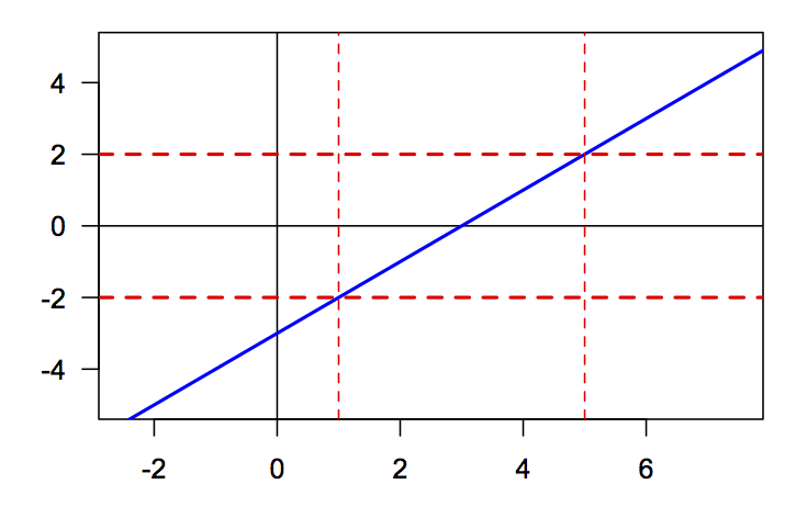
We see that the graph \(y=x-3\) is between the two thresholds when \(x\) is between 1 and 5. \[ \{x : |x-3| < 2\} = \{x : 1 < x < 5\} = (1,5). \]

A third approach is to view \(|x-3|\) as the distance between the expressions \(x\) and \(3\). This is similar to the first approach, except that instead of thinking about \(x\) and \(3\) as numbers on a number line, we will graph both expressions \(y=x\) and \(y=3\). We seek to find values \(x\) so that the distance between these graphs is less than 2. We do this by also graphing threshold curves that show when we are within the desired distance.

For example, we could consider \(y=3\) as the reference value so that the threshold curves are found by adding and subtracting 2 to get \(y=5\) and \(y=1\). We are now interested in when the other expression \(y=x\) is found between the threshold curves.

We see that the graph \(y=x\) is between the two thresholds \(y=1\) and \(y=5\), meaning less than a distance 2 from \(y=3\), when \(x\) is between 1 and 5. \[ \{x : |x-3| < 2\} = \{x : 1 < x < 5\} = (1,5). \]

However, we could also consider \(y=x\) as the reference value and the threshold curves are found by adding and subtracting to 2 get \(y=x+2\) and \(y=x-2\) as the thresholds. We then seek to find where the other expression \(y=3\) is found between these thresholds.

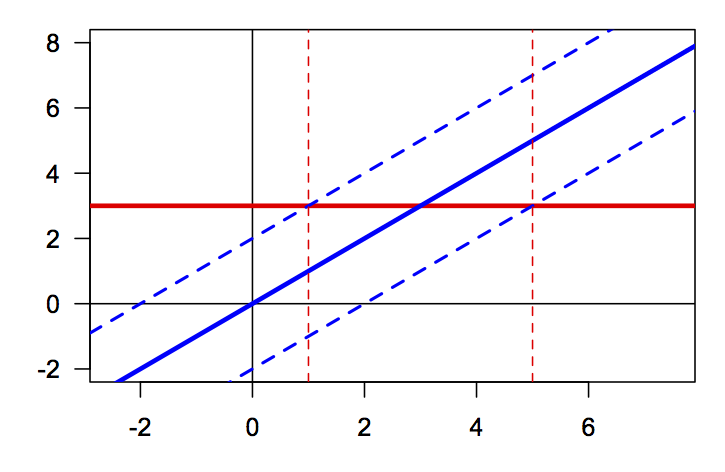
Of course, it is no surprise that we find the same solution set, \[ \{x : |x-3| < 2\} = \{x : 1 < x < 5\} = (1,5). \]

Example: Use a graph to determine the solution set \(\{x : |x^2+5x|>1\}\) using interval notation.

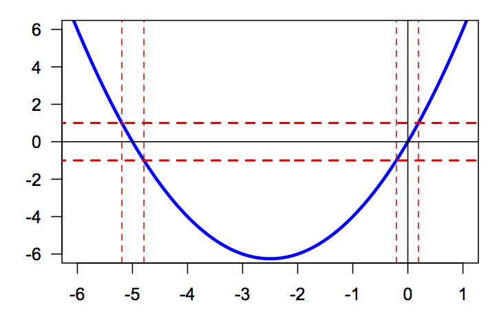
We can consider this problem in three different ways, each of which will give the same result. The first is to consider a single expression \(y=x^2+5x\) and determine when this graph is outside the band of thresholds that are found 1 unit away from the horizontal axis, \(y=0\). Graphically, we see when \(y=x^2+5x\) is outside both \(y=-1\) and \(y=1\).

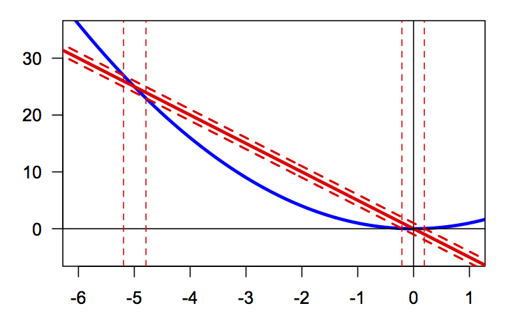
The other approaches require that we consider \(x^2+5x\) as a difference, which requires introducing an additive inverse, \(x^2+5x = x^2 - -5x\). Then we consider the graphs \(y=x^2\) and \(y=-5x\), and we want to know when the distance between these values is more than 1 unit. One approach is to see when \(y=-5x\) is outside the band formed by \(y=x^2-1\) and \(y=x^2+1\). Or we can see when \(y=x^2\) is outside the band formed by \(y=-5x-1\) and \(y=-5x+1\).

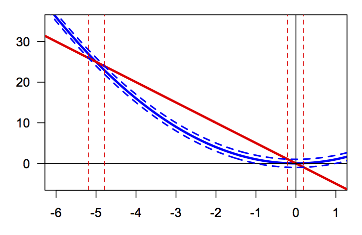
Although the pictures of these different threshold bands look somewhat different, the locations where the various curves cross the thresholds are always the same. These points are found as the solutions to the equations \[x^2+5x=-1 \qquad \hbox{or} \qquad x^2+5x=1.\] To solve these equations, we need to move everything to one side so the equation is an expression equals zero, \[x^2+5x+1=0 \qquad \hbox{or} \qquad x^2+5x-1=0.\] Both of these are quadratic equations, which are solved using the quadratic formula to find the four points, \[x=\frac{-5\pm\sqrt{21}}{2} \qquad \hbox{or} \qquad x=\frac{-5\pm\sqrt{29}}{2}.\] Ordering these values left to right, we can identify how the values relate to the graph, \[ \frac{-5-\sqrt{29}}{2} < \frac{-5-\sqrt{21}}{2} < \frac{-5+\sqrt{21}}{2} < \frac{-5+\sqrt{29}}{2}.\] The solution to the inequality involves three disjoint intervals, so that the solution set is the union \[ (-\infty,\frac{-5-\sqrt{29}}{2}) \cup (\frac{-5-\sqrt{21}}{2},\frac{-5+\sqrt{21}}{2}) \cup (\frac{-5+\sqrt{29}}{2},\infty).\]