Mathematicians seek to establish a body of knowledge that is built on principles of logic.
As such, the idea of a definition to a mathematician is more precise than being
merely an explanation of the idea or the meaning of the idea. To a mathematician,
definitions are given for properties that will be attributed to objects
and the definition provides a logical statement that characterizes whether the property
applies or not.
For example, consider what it means to say that a set \(S\) of points in the plane is linear.
In the sense of natural language, we might say that the set is straight. In the
sense of mathematics, the idea of linear is a property of a set that captures the idea
that the slope between any two points is always the same. We can formally describe the
property if we create a logical statement that matches this idea.
There exists a single value \(m\) (possibly infinite) so that for any points
\(P_1 = (x_1,y_1) \in S\) and \(P_2=(x_2,y_2) \in S\), if \(P_1 \ne P_2\)
then \(\displaystyle m = \frac{y_2-y_1}{x_2-x_1}\). (Use \(m=\infty\) if \(x_1=x_2\).)
In a loose sense, we could think of this logical statement as a true/falsefunction
of a set, maybe named \(\mathrm{IsLinear}\). When we take a set \(S\) as an input to the statement,
we check whether \(\mathrm{IsLinear}(S)\) is true or false. When it is true, we are
allowed to use the phrase \(S\) is linear. Otherwise, we are obligated
to say \(S\) is not linear.
A Mathematical Definition of Limit
When we think about a limit of a function at a point \(c\), we think about a value
\(L\) that the output of a function approaches when the input approaches \(c\), perhaps
written as \(f(x) \to L\) as \(x \to c\). As an equation, we write
\[ \lim_{x \to c} f(x) = L. \]
That is, we want to think of a limit as a mathematical object representing a value.
Unfortunately, there is not a single rule for how to find the value for limit. So
a definition can not be based on how the value is found.
Mathematics requires that we define things using logical statements.
In this case, there are three related objects that go into the definition: the function,
the input limit \(c\), and the output limit \(L\).
So the definition of a limit is actually based on a rule to determine whether we should
consider the equation
\[ \lim_{x \to c} f(x) = L \]
is true or false. That is, for the purposes of the definition, we do not think about the
limit in terms of finding its value; we think about what is required for the combination
\(f(x)\), \(c\) and \(L\) to make the equation for the limit true.
So for a function or expression \(f(x)\), an input value \(c\), and an output value \(L\),
we wish to create a logical statement (essentially a true/false function,
say \(\mathrm{IsLimit}(f(x),c,L)\)) that captures whether or not \(L\) is the appropriate
limit for \(f(x)\) when \(x \to c\). The standard definition for a limit provides this
logical test for the triple \((f(x), c, L)\).
For every value \(\epsilon > 0\), there exists some value \(\delta > 0\) such that
if \(x \ne c\) and \(|x-c| < \delta\) then \(|f(x)-L| < \epsilon\).
Ordinarily, the statements \(x \ne c\) and \(|x-c| < \delta\) are combined as
\(0 < |x-c| < \delta\).
In this definition (the rule to test \(\mathrm{IsLimit}\)), the use of absolute value
captures the idea of distance or accuracy of approximation. We should view
the two measures of distance (one for \(x\) and one for \(f(x)\)) as characterizing
two sequences. An input sequence \(x_n\) gives us values for \(x = x_1, x_2, x_3, \ldots\),
which eventually move closer and closer to \(c\),
while the function creates an output sequence \(y_n = f(x_n)\). For \(L\) to be the
limit of the approximations \(y_n\), the values \(y_n\) must get closer and closer to \(L\).
The relationship between \(\epsilon\) (epsilon) and \(\delta\) (delta) provides a connection
between how close we need the values \(x_n\) to be to \(c\) in order to guarantee
that the values of \(y_n\) are close enough to \(L\). The value \(\epsilon\) gives
us the requested accuracy between \(y_n\) and \(L\). The value \(\delta\) (which usually
depends on \(\epsilon\)) tells us how close to make \(x_n\) from \(c\) to accomplish
the \(\epsilon\)-accuracy for \(f(x)\).
Subsets and Visualizing the Definition
The implication \( 0 < |x-c| < \delta \Rightarrow |f(x)-L| < \epsilon\) can be interpreted
as a statement about subsets. Suppose \(\delta\) and \(\epsilon\) are fixed numbers.
The inequality \(0 < |x-c| < \delta\) has a solution set that is sometimes called a
punctured neighborhood of \(c\) given by \(N(c,\delta)=(c-\delta, c) \cup (c, c+\delta)\).
We could also solve the inequality \(|f(x)-L| < \epsilon\) and obtain its solution set.
The implication tells us that for every \(x\) in the punctured neighborhood, that \(x\)
must also be in the solution set. So the punctured neighborhood is a subset
of the solution set to \(|f(x)-L| < \epsilon\).
(Illustration of a punctured neighborhood, \(N(c,\delta)\))
The inequality \(|f(x)-L| < \epsilon\) is related to the inequality \(|y-L| < \epsilon\),
which in the \((x,y)\)-plane corresponds to a horizontal band between \(y=L-\epsilon\)
and \(y=L+\epsilon\). The solution set to \(|f(x)-L| < \epsilon\) corresponds to the
set of \(x\)-values for which \(y=f(x)\) appears inside this horizontal band. In other words,
\(f(x)\) is between the thresholds of \(L-\epsilon\) and \(L+\epsilon\).
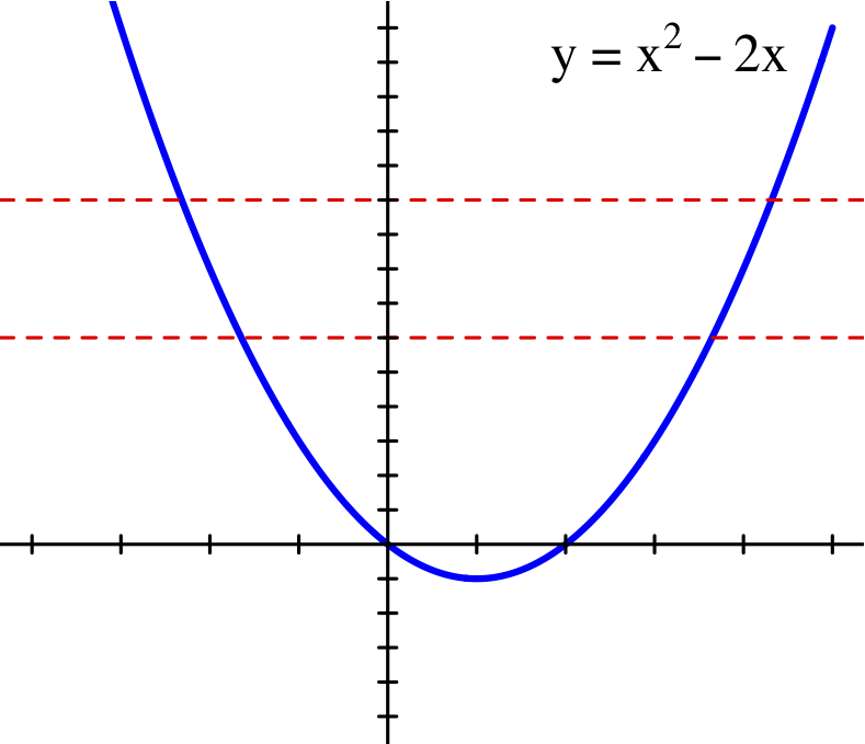
Example: Consider \(f(x) = x^2 - 2x\). Since \(f(4)=8\), we expect
\[ \lim_{x \to 4} f(x) = 8. \]
This example will illustrate the relationships between the punctured neighborhoods of \(c=4\)
and the threshold bands around \(L=8\).
A graph of \(y=f(x)\) along with threshold bands around \(y=8\) with \(\epsilon = 2\) is
illustrated. The solution set to \(|f(x)-8| < 2\), which is a union of two intervals,
can be found by solving for the intersection points with the function and the threshold lines,
\[
\begin{align*}
x^2-2x &= 6 \qquad &\Leftrightarrow \qquad x &= 1 \pm \sqrt{7}, \\
x^2-2x &= 10 \qquad &\Leftrightarrow \qquad x &= 1 \pm \sqrt{11}. \\
\end{align*}
\]
So the solution set is \((1-\sqrt{11}, 1-\sqrt{7}) \cup (1+\sqrt{7}, 1+\sqrt{11})\),
which to 4 decimal places is approximately \((-2.3166,-1.6458) \cup (3.6458, 4.3166)\).
This solution set is illustrated below using a marked number line.
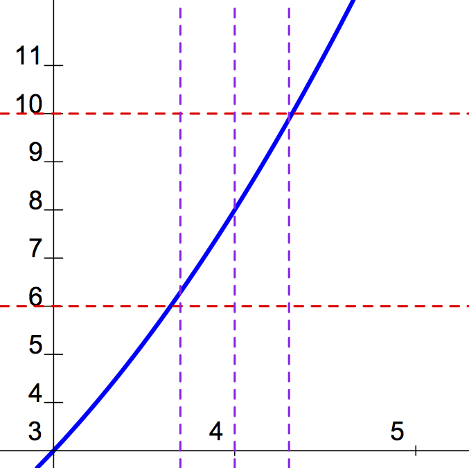
Notice that one of the intervals contains our reference point \(c=4\).
We will now focus only on that subinterval and look at the punctured neighborhoods
around \(c=4\). Notice that \(N(4,\delta=0.2)\) is a subset while \(N(4,\delta=0.4)\)
is not.
Consequently, we have just seen that the inequality \(|f(x)-8| < 2\) is true
whenever \(x \in N(4,\delta=0.2)\), or in other words \(0 < |x-4| < 0.2\).
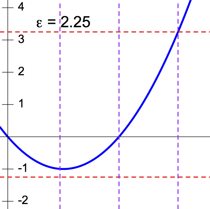
The value of \(\delta\) that we found is not the largest possible value that works.
Because the solution set includes the entire interval \((1+\sqrt{7},1+\sqrt{11})\),
we might seek the largest value of \(\delta\) so that
\(N(4,\delta) \subseteq (1+\sqrt{7},1+\sqrt{11})\).
An approximate answer is easily seen using decimal approximations and seeing how far
each end-point is from the neighborhood center at \(c=4\).
\[
\begin{align*}
|4 - (1+\sqrt{7})| &\approx |4 - 3.6458| = 0.3542 \\
|4 - (1+\sqrt{11})| &\approx |4 - 4.3166| = 0.3166
\end{align*}
\]
Let us look at the corresponding punctured neighborhoods.
We see that the smaller distance from 4 to the solution's edge gives the
size of the largest punctured neighborhood that remains completely inside
the solution set.
So the largest value of \(\delta\) that makes \(N(4,\delta) \subseteq (1+\sqrt{7},1+\sqrt{11})\)
is \(\delta_\max = \sqrt{11}-3 \approx 0.3166\).
The most common way of visualizing this relationship between the \(\epsilon\)-inequality
and the \(\delta\)-neighborhood is to show the \(y = L \pm \epsilon\) thresholds with
the graph \(y=f(x)\). Then add vertical lines at the edges of the punctured
neighborhood, at \(x=c \pm \delta\) and \(x=c\). The subset relation will be true,
as needed, if the graph \(y=f(x)\) is contained between the \(\epsilon\)-thresholds
for each \(x\) in the punctured neighborhood. For the previous example, the
illustration would be as given to the right. If \(\delta\) is chosen too large, then the
graph \(y=f(x)\) will appear above or below the thresholds.
The Relationship between Delta and Epsilon
So far, we have considered a particular value for \(\epsilon\) and focused on what
values of \(\delta\) make the implication
If \(0 < |x-c| < \delta\) then \(|f(x)-L| < \epsilon\)
a true statement. That is, the punctured neighborhood of size \(\delta\) is a subset
of the solution set,
\[ N(c,\delta) = \{ x : 0 < |x-c| < \delta \} \subseteq \{ x : |f(x)-L| < \epsilon \}. \]
In the limit definition of a limit, we are interested in the set of all possible
choices of \(\epsilon\) and \(\delta\) that make this true.
So consider the pairs \((\epsilon, \delta)\) that satisfy the limit implication for
a given function \(f(x)\), point \(c\) and value \(L\),
\[ \{ (\epsilon, \delta) : 0 < |x-c| < \delta \Rightarrow |f(x)-L| < \epsilon \}. \]
The limit definition tells us that \(f(x) \to L\) as \(x \to c\) if
for every \(\epsilon > 0\), there will be a value \(\delta > 0\) so that
\((\epsilon, \delta)\) is in this set where the implication is true.
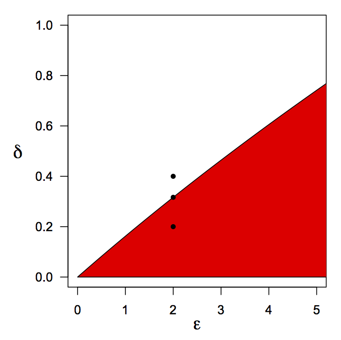
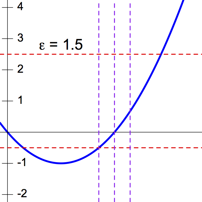
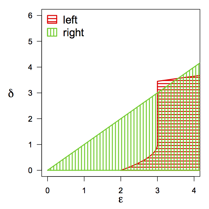
Example: Using the same function \(f(x)=x^2-2x\), \(c=4\) and \(L=8\),
visualize and interpret the set
\[ \{ (\epsilon, \delta) : 0 < |x-4| < \delta \Rightarrow |(x^2-2x) - 8| < \epsilon \}. \]
The set of \((\epsilon, \delta)\) is shown to the right.
For example, the case where \(\epsilon = 2\) is the example we studied above.
The three points illustrated with \(\epsilon = 2\) correspond to the three cases we analyzed.
The point \(2, 0.4\) is not in the set because we saw that
\(N(4,0.4) \not \subseteq \{ |f(x)-8| < 2 \}\).
The point \(2, 0.2\) is in the set because \(N(4,0.2) \subseteq \{ |f(x)-8| < 2 \}\).
The highest point with \(\epsilon=2\) is \((2, \sqrt{11}-3)\), which is also in the set.
Notice that for the function \(f(x)=x^2-2x\), \(c=4\) and \(L=8\), the set of
\((\epsilon, \delta)\) making the limit implication true includes points for
every \(\epsilon > 0\). This is the meaning of the definition of the limit
statement
\[ \lim_{x \to 4} [ x^2-2x ] = 8 \]
which is the logical statement
For every \(\epsilon > 0\), there exists a value \(\delta > 0\)
so that \(0 < |x-4| < \delta\) implies \(|(x^2-2x) - 8| < \epsilon\).
In order to understand how the limit definition is mathematically meaningful,
it is useful to explore some examples where a value \(L\) is not the limit value.
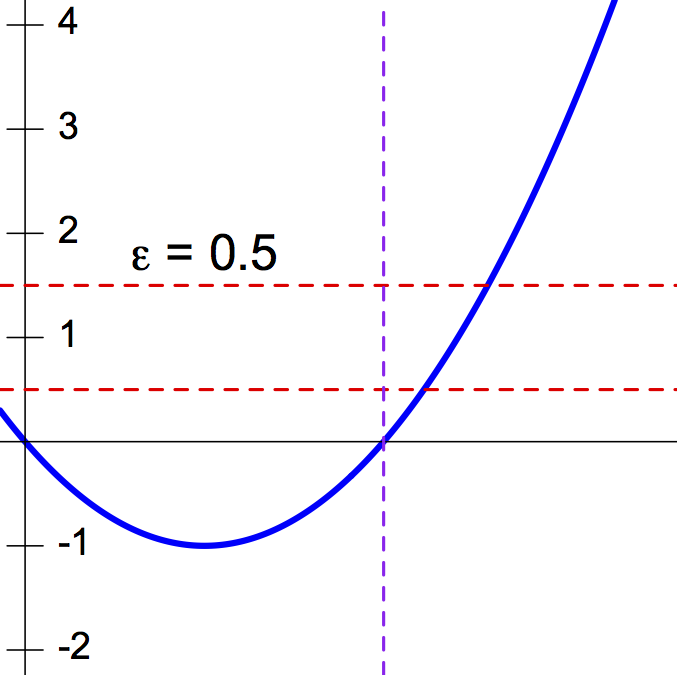
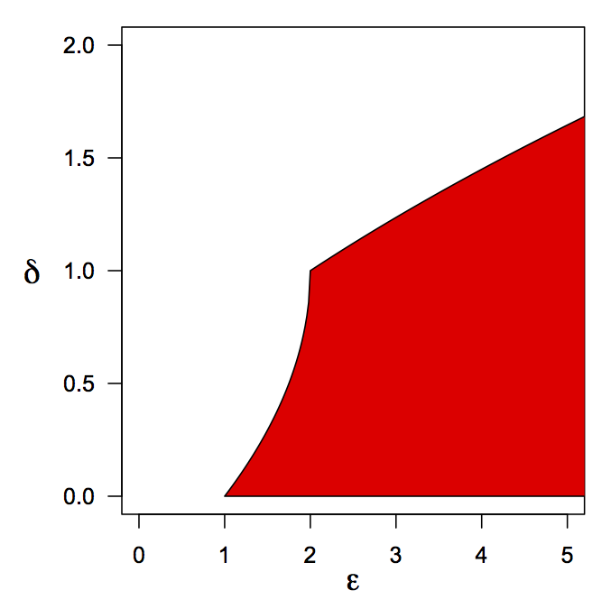
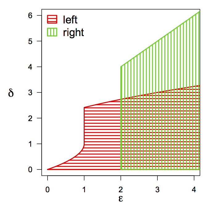
Example: Using the function \(f(x)=x^2-2x\), \(c=2\) and \(L=1\), visualize
and interpret the set
\[ \{ (\epsilon, \delta) : 0 < |x-2| < \delta \Rightarrow |(x^2-2x) - 1| < \epsilon \}. \]
The actual limit should have been \(f(2) = 2^2-2(2)=0\). So when we draw thresholds,
if \(\epsilon\) is small enough, the graph \(y=f(x)\) is not going to be between the lines
at \(y=1 \pm \epsilon\) for any punctured neighborhood of \(c=2\). It may be possible that
when \(\epsilon\) is large enough, there will be some overlap.
The three graphs below illustrate three different situations. When \(\epsilon < 1\),
the solution set to \(|f(x)-1| < \epsilon\) is completely away from \(x=2\).
So there are no punctured neighborhoods of \(x=2\) that are subsets of the solution.
When \(1 < \epsilon < 2\), the solution set \(\{|f(x)-1| < \epsilon\}\) is the union
of two intervals and the right-most interval does contain a
neighborhood of \(x=2\). Finally, when \(\epsilon > 2\), the set \(\{|f(x)-1|<\epsilon\}\)
is a single connected interval which contains neighborhoods of \(x=2\).
The relation of all pairs \((\epsilon, \delta)\) such that the limit implication
\[ 0 < |x-2| < \delta \Rightarrow |(x^2-2x) - 1| < \epsilon \]
is true is shown to the right.
Because there are no points with \(\epsilon < 1\) in this set, \(L=1\) is
clearly not the limit of \(f(x)\) as \(x \to 2\).
Question: Based on the graphs above, you should be able to find formulas that describe
the boundary of the relation for \((\epsilon, \delta)\) by using the quadratic formula
to find intersection points, and then using these solutions to compute \(\delta\).
What are the formulas?
The previous example illustrated what happens when you have the wrong value for the limit.
For a piecewise function with a jump discontinuity, we have this problem on one side
but not the other, as illustrated in the next example.
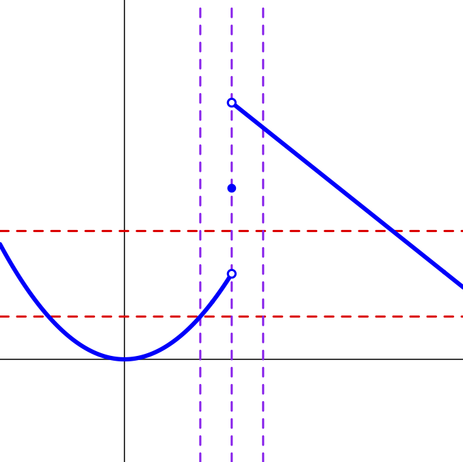
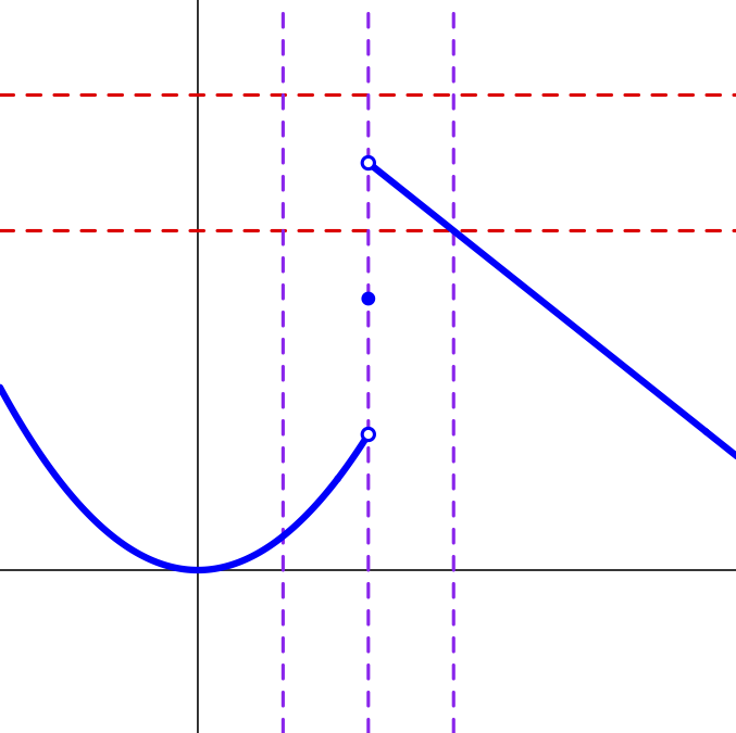
Example: The piecewise function \(f\) defined below has no limit at \(x=1\)
because the left- and right-limits disagree.
\[ f(x) = \begin{cases}
x^2, & x < 1, \\
2, & x = 1, \\
4-x, & x > 1.
\end{cases}
\]
Suppose we thought the limit at \(x=1\) was based on the formula \(x^2\) so that \(L=1^2 = 1\).
Let us explore the inequality \(|f(x) - 1| < \epsilon\) for small \(\epsilon\).
The graph of \(y=f(x)\) along with thresholds around \(L=1\) using \(\epsilon = 0.5\)
is illustrated to the right.
Because of the jump in the function, the solution to \(|f(x)-L|<\epsilon\) does not
include a punctured neighborhood of \(x=1\). (If \(\epsilon\) is made large enough,
there will be an included neighborhood; but a limit requires a neighborhood for all
values of \(\epsilon\) no matter how small.)
So \(L=1\) is not the limit.
However it does include a left-neighborhood, \((1-\delta, 1)\),
with \(\delta = 1-\frac{1}{\sqrt{2}} \approx 0.293\).
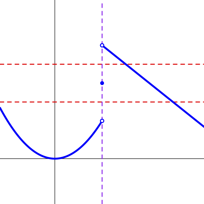
Next, suppose we thought the limit at \(x=1\) was based on the formula \(4-x\)
so that \(L=4-1 = 3\).
If we explore the inequality \(|f(x) - 3| < \epsilon\) for small \(\epsilon\),
again using \(\epsilon = 0.5\), then we need to consider the graph of \(y=f(x)\)
and the thresholds around \(L=3\) using \(\epsilon = 0.5\) as shown to the right.
Again because of the jump in the function, the solution to \(|f(x)-L|<\epsilon\) does not
include any punctured neighborhood of \(x=1\).
So \(L=3\) is not the limit.
Yet this time, the inequality solution includes a right-neighborhood, \((1, 1+\delta)\),
with \(\delta = 0.5\).
Finally we might think the limit at \(x=1\) is just the value \(L=f(1)=2\).
So we explore the inequality \(|f(x) - 2| < \epsilon\).
The graph of \(y=f(x)\) along with thresholds around \(L=2\) using \(\epsilon = 0.5\)
is shown.
This time, we are not using a value matching either the left or the right side.
So the solution to \(|f(x)-L|<\epsilon\) does not include a neighborhood to the
left or to the right of \(x=1\), let alone a punctured neighborhood around \(x=1\).
Consequently, \(L=2\) is also not the limit.
This function has no limit at \(x=1\) since the inequality
\(|f(x)-L| < \epsilon\) for any value of \(L\) will not include a punctured neighborhood
around \(x=1\).
However, for \(L=1\), the inequality will have a left interval \((1-\delta, 1)\)
that is in the solution set.
For this reason, we say that \(L=1\) is a left-limit of \(f(x)\) at \(x=1\),
which is written
\[ \lim_{x \to 1^-} f(x) = 1. \]
Similarly, for \(L=3\), the inequality will have a right interval \((1,1+\delta)\)
that is in the solution set.
Thus, we say that \(L=3\) is a right-limit of \(f(x)\) at \(x=1\), written
\[ \lim_{x \to 1^+} f(x) = 3. \]
We now consider the relation of values \((\epsilon, \delta)\) that make the limit
implication true, except that we consider the left and right neighborhoods separately.
In particular, the left-limit implication corresponds to the logical statement
\[ x < 1 \hbox{ and } |x-1|<\delta \quad \Rightarrow \quad |f(x)-L| < \epsilon. \]
The right-limit implication corresponds to the logical statement
\[ x > 1 \hbox{ and } |x-1|<\delta \quad \Rightarrow \quad |f(x)-L| < \epsilon. \]
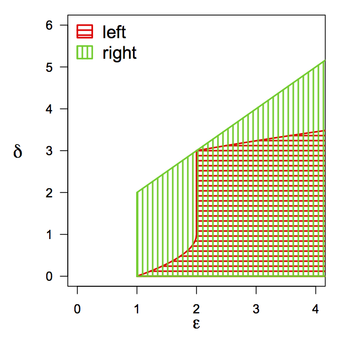
For the value \(L=1\), which is the limit on the left, we see that the relation
between \(\epsilon\) and \(\delta\) includes points for all values of \(\epsilon > 0\),
but only for the left-limit implication. That is, for every value \(\epsilon > 0\),
there are values \(\delta > 0\) so that \((1-\delta, 1)\) is a subset to the solution
\(|f(x)-1| < \epsilon\). The right-limit implication is not satisfied
for small values of \(\epsilon\).
For the value \(L=3\), which is the limit on the right, we see that the relation
between \(\epsilon\) and \(\delta\) includes points for all values of \(\epsilon > 0\),
but only for the right-limit implication. That is, for every value \(\epsilon > 0\),
there are values \(\delta > 0\) so that \((1, 1+\delta)\) is a subset to the solution
\(|f(x)-1| < \epsilon\). This time, the left-limit implication is not satisfied
for small values of \(\epsilon\).
For the value \(L=2\), which is the value of the function \(f(1)=2\), this value
is neither a left-limit or a right-limit. The relation shows that for small values
of \(\epsilon\), namely \(\epsilon < 1\), there are no values \(\delta > 0\)
so that either the left or right intervals satisfy the inequality \(|f(x) - 2| < \epsilon\).