Limits and Approximations
The most important applications of limits relate to performing a calculation that can not be done at a point of interest, but which can be done at nearby points. A limit corresponds to the extrapolation of all approximations to a point of interest without testing the actual point of interest.
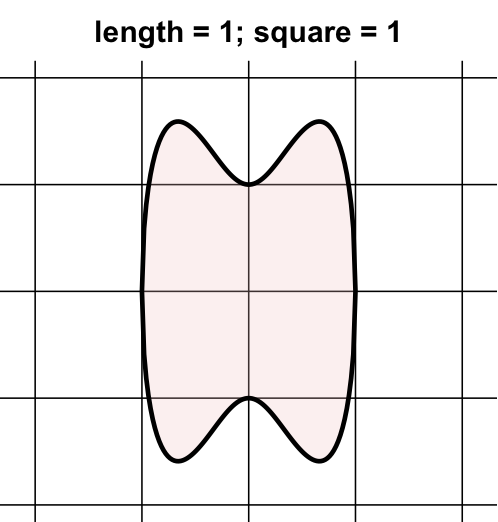
As a first mathematical example, consider the task of finding the area of the region illustrated in the figure to the right. Because the shape is curved, there are no simple geometric rules to find the answer.
Instead, we can estimate the area by measuring the area of all squares that contain a portion of the region. In our image, the region is in part of 8 of the squares. Each illustrated square has an area of 1 square unit, so that our approximation of the area is 8 square units. If the squares are too big (which is the case for our image), this approximation is not very good.
But if we use small enough squares, the approximation will be reasonable. The image below has a dynamic control where you can set the size of the squares, and squares that are identified as overlapping with the shape are identified and counted. Try varying the size of the squares as well as choosing if a portion or the entire square must be included — see how this affects the approximation of the area.
This example illustrates many of the key ideas of a limit. We are approximating a quantity (the area) by measuring the area of squares that are either partially or entirely within the region of interest. The approximation improves when we make the size of the squares smaller, although that makes the actual counting take longer. We imagine that if we could make the squares smaller and smaller, our approximation would get as close to the real area as possible. That is, the true area is the limit of the approximations.
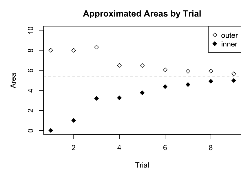
Let us organize our observations. Suppose we create a list of approximation trials. We can summarize our results in a table, or in a graph.
| Trial | Size | Outer Area | Inner Area |
|---|---|---|---|
| 1 | 1 | 8 | 0 |
| 2 | 0.5 | 8 | 1 |
| 3 | 0.4 | 8.32 | 3.2 |
| 4 | 0.25 | 6.5 | 3.25 |
| 5 | 0.2 | 6.48 | 3.76 |
| 6 | 0.125 | 6.0625 | 4.375 |
| 7 | 0.1 | 5.9 | 4.58 |
| 8 | 0.075 | 5.9175 | 4.905 |
| 9 | 0.05 | 5.65 | 4.98 |
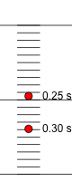
As a second example of thinking of limits as the extrapolation of progressively better approximations, we consider the challenge of measuring the velocity of a falling object using high-speed photography. An average velocity can be computed by measuring the distance travelled and dividing by the time elapsed between images. The reason this is a challenge is that gravity makes the object continuously increase in speed, so our calculated average velocity will depend on how much time is allowed between images.
After 1/4 second, a falling object has travelled 1 foot. We wish to see how fast the object is moving at that instant. If we capture an image of the object at 1/4 second (\(t=0.25\) s) and again 1/20 second later (\(t=0.30\) s), and then overlay the images to measure distance travelled, we can compute the distance. The height of the ball (relative to starting height) at \(t=0.25\) s is \(y=-1.00\) ft. At the second moment, \(t=0.50\) s, the height is \(y=-1.44\) ft. If we introduce the symbol \(v_{[0.25,0.30]}\) for the average velocity over the time interval from \(t=0.25\) s to \(t=0.30\) s, this average velocity can be computed as \[v_{[0.25,0.30]} = \frac{(-1.44 - -1.00) \hbox{ ft}}{(0.30 - 0.25) \hbox{ s}} = \frac{-0.44 \hbox{ ft}}{0.05 \hbox{ s}} = -8.8 \hbox{ ft/s}.\]
Of course, this is just one approximation of the velocity. We could repeat the experiment, taking the second snapshot with a shorter delay. The dynamic activity below allows you to choose the delay for the second snapshot and shows the relevant measurements and calculations. While you are exploring the calculations, you should also explore the importance of measurement accuracy.
Questions for Reflection
- If you set the delay to \(\Delta t = 0.005\) s, what is the average velocity? Would it be correct or incorrect to say this is the velocity of the ball at the instant \(t=0.25\) s? Why?
- If you set the delay to \(\Delta t = 0.005\) s, what is the reported average velocity for different choices of measurement precision? Repeat the process for \(\Delta t = 0.002\) s.
- Based on the previous question, in general terms, how does the required measurement precision relate to the delay between measurements?
In the previous activity, we computed average velocities over intervals in order to approximate the velocity of the ball at the instant \(t=0.25\) s. We noticed that if our measurement precision was not great enough, when the delay was particularly short, the difference between observations was not accurate and we obtained rather faulty approximations. However, when the precision of observations was increased, we found that the average velocities seemed to be steadily getting closer to a velocity of \(v=-8.0\) ft/s. If this is really the case (and it would require further calculations to explore), the velocity -8 ft/s would be the limit of our approximations.
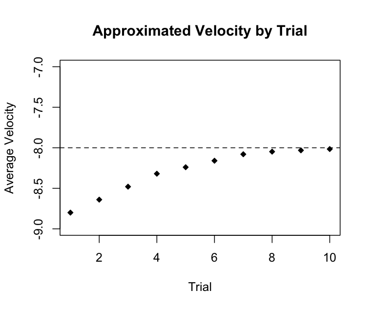
Similar to our earlier example, let us organize our observations. While we might have just watched the computed average velocities as we moved the slider for the delay between observations to find a pattern, for a table and a graph, we need to consider a sequence of individual observations. One possible collection of ever-improving approximations is given below (using maximum available precision). If you were to create a different sequence of trials, the particular numbers you would obtain would differ from those shown. But the overall pattern would persist, with the sequence of approximations steadily moving closer to the limiting value at \(v=-8.0\) ft/s.
| Trial | Delay (s) | Average Velocity (ft/s) |
|---|---|---|
| 1 | 0.05 | -8.8 |
| 2 | 0.04 | -8.64 |
| 3 | 0.03 | -8.48 |
| 4 | 0.02 | -8.32 |
| 5 | 0.015 | -8.24 |
| 6 | 0.01 | -8.16 |
| 7 | 0.005 | -8.08 |
| 8 | 0.003 | -8.048 |
| 9 | 0.002 | -8.032 |
| 10 | 0.001 | -8.016 |
Our objective was to recognize limits as extrapolating a sequence of approximations. In both examples above, we were working with calculations for which the physical process was not defined for the limiting case.
In the first example, we were adjusting the grid size. For positive numbers, such a grid actually existed and we could compute area. Our limiting approximation was steadily making the grid size closer and closer to zero. But a grid size of zero makes no physical sense.
In the second example, we were adjusting the delay between observations. For a positive delay, we had two distinct times and we could compute an average velocity over the interval. Our limiting approximation was steadily making the delay closer and closer to zero. However, a delay of zero would have corresponded to no time elapsed between measurements making an average velocity calculation meaningless.
While these two examples physically made it impossible to perform the calculation at the limiting state, this is not always the case. Nevertheless, in order to maintain a consistent view of things, when performing limits, we will always take the view that the limit is the extrapolation of values as our trials steadily get closer to the limiting state as if the limiting state itself could never be used. If we can compute the value at the limiting state, then the question becomes one of whether the extrapolation of approximations will agree with the actual value at the limiting state.
In the next section, we will take a new perspective of our approximations. In the examples above, our tables and graphs summarizing the sequence of approximations focused on the sequence of trials themselves. On our graph, this led to the perspective that the approximations were moving closer to the horizontal limiting line as we performed more and better approximations. The new perspective will consider the relation between the independent variable (what we controlled) and the dependent variable (the approximating calculation).