The most intuitive place to use limits is for piecewise functions.
To start, let us consider a function defined piecewise like
\[
f(x) = \begin{cases}
x^2, & x < 1, \\
3, & x = 1, \\
x+1, & x > 1.
\end{cases}
\]
When we write \(f(1)\), this has only one possible meaning — the output value
of the function when the input is 1, which is \(f(1) = 3\). But we very often
need to know what the other two formulas would have given if they had been
used. This is the most basic interpretation of what a limit computes.
A limit is an extrapolation of an approximation to a point of interest.
So if \(f(x)\) is a function or expression in the variable \(x\) and
we are interested in a point \(a\), we can use \(f(x)\) with points \(x < a\)
as approximations (on the left) or with points \(x > a\) as approximations
(on the right).
If we use the points on the left for our approximations, we write
\[\lim_{x \to a^-} f(x),\]
and if we use the points on the right for our approximations, we write
\[\lim_{x \to a^+} f(x).\]
When the value does not depend on which side we use, we can drop the ±
and simply write
\[\lim_{x \to a} f(x).\]
Example: For the piecewise function
\[
f(x) = \begin{cases}
x^2, & x < 1, \\
3, & x = 1, \\
x+1, & x > 1,
\end{cases}
\]
demonstrate how to evaluate the formulas \(x^2\) and \(x+1\) at \(x=1\).
We can not use the notation \(f(1)\), since that can only refer to the value
\(f(1)=3\). To use the formula \(x^2\), which is used for \(x < 1\), we use the
left limit,
\[ \lim_{x \to 1^-} f(x) = 1^2 = 1. \]
To use the formula \(x+1\), which is used for \(x > 1\), we use the right limit,
\[ \lim_{x \to 1^+} f(x) = 1+1 = 2. \]
Because these two one-sided limits are different, we can not talk about
\(\lim_{x \to 1} f(x)\) since this is only used when the two sides go to the same value.
We say that the two-sided limit does not exist.
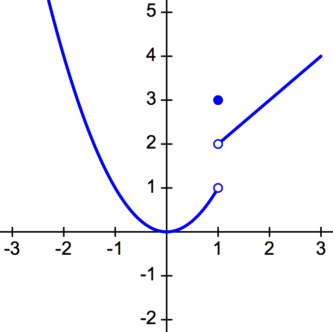
If we look at a graph of \(y=f(x)\), we see that the value and limits of the function
have different roles. The value of the function, \(f(1)\) represents the actual
point (solid) that aligns with the vertical line \(x=1\). The left-limit
\(\displaystyle \lim_{x \to 1^-} f(x) = 1\) represents the extrapolated end-point
for the branch of \(f(x)\) for \(x < 1\), which is often shown as an empty point.
Similarly, the right-limit \(\displaystyle \lim_{x \to 1^+} f(x) = 2\) represents
the extrapolated end-point for the branch of \(f(x)\) for \(x > 1\).
When the branches on the left or right approach a vertical asymptote, the limit
does not really exist; but we use infinity notation to indicate if the increases
or decreases without bound. For rational functions (quotients of polynomials),
the easiest way to determine the limits algebraically is by performing a sign-analysis
summary of the function.
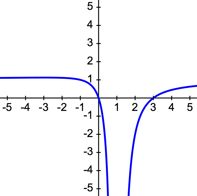
Example: Use limits to describe the vertical asymptote of
\[f(x) = \frac{x^2-3x}{x^2-2x+1}.\]
Before doing anything else, we need to factor our formula,
\[ f(x) = \frac{x(x-3)}{(x-1)(x-1)}. \]
We see that the two factors in the denominator are the same, \(x-1\), and since
\(\div(x-1)\) is undefined for \(x=1\), our function has a vertical asymptote at \(x=1\).
(Note: This only works when the function has been simplified. Since \(x-1\) is not a
factor in the numerator, this function has already been simplified.)
Now we do a sign analysis using these factors. Note that because \(x-1\) was a double
factor, the sign does not change when we cross \(x=1\).
\(\displaystyle \frac{x(x-3)}{(x-1)(x-1)}\)
Because \(f(x)\) has a vertical asymptote at \(x=1\) and the sign analysis shows that
\(f(x)\) is negative on each side of \(x=1\), on the intervals \((0,1)\) and \((1,3)\),
we say the limits on the left and right go to \(-\infty\),
\[
\begin{align*}
\lim_{x \to 1^-} f(x) = -\infty, \\
\lim_{x \to 1^+} f(x) = -\infty.
\end{align*}
\]
In this case that both one-sided limits are the same, we can use a single limit
symbol to represent both sides at once,
\[ \lim_{x \to 1} f(x) = -\infty. \]
Limits and Continuity
For elementary problems in calculus, the functions are basic algebraic functions.
These functions have the important property of being continuous. This means
that as long as a function (think: formula) is defined at a point, the limit
(the extrapolation of approximations from the sides) agrees with the function,
\[\lim_{x \to c} f(x) = f(c).\]
This means that the limits for algebraic functions can be computed if we can
find an equivalent formula that is defined at the point of interest.
Example: Evaluate the limit \(\displaystyle \lim_{x \to 3} x^2\).
The function \(f(x)=x^2\) is continuous. So when computing a limit, we get to use
the same formula. That is, we could think of the function as a piecewise
function using the same formula for all pieces,
\[ f(x) = \begin{cases}
x^2, & x < 3, \\
x^2, & x = 3, \\
x^2, & x > 3
\end{cases} \]
So the one-sided limits, which give the extrapolation of approximations
from the sides, use \(x^2\),
\[
\begin{align*}
\lim_{x \to 3^-} f(x) &= 3^2 = 9, \\
\lim_{x \to 3^+} f(x) &= 3^2 = 9.
\end{align*}
\]
Since the two one-sided limits agree, we can write the limit without
reference to sides,
\[ \lim_{x \to 3} f(x) = 3^2 = 9. \]
In an example like this, where the same formula is used for \(x < c\) and for \(x > c\),
we can simply compute the two-sided limit rather than show the one-sided limits.
Example: Evaluate the limit \(\displaystyle \lim_{x \to 1} \frac{x}{x-2}\).
Since the function \(f(x) = x \div(x-2)\) is defined at \(x = 1\), we can use
continuity and evaluate the limit using the same formula,
\[ \lim_{x \to 1} \frac{x}{x-2} = \frac{1}{1-2} = -1. \]
When an algebraic function is not defined at \(x = c\), then we should see
if a simplified version of the formula is defined at the point. If so,
the original function had a hole at the point and we can compute the limit.
Example: Evaluate the limit \(\displaystyle \lim_{x \to 2} \frac{x^2-2x}{x^2-4}\).
This time, the function \(f(x) = (x^2-2x) \div (x^2-4)\) is not defined at \(x=2\).
So we factor the formula and see if it simplifies.
\[ f(x) = \frac{x^2-2x}{x^2-4} = \frac{x(x-2)}{(x+2)(x-2)} = \frac{x}{x+2}, \quad x \ne 2. \]
That is, the original function is not defined at \(x=2\), so the simplified formula is
really a piecewise function,
\[ f(x) = \begin{cases}
\frac{x}{x+2}, & x < 2, \\
\frac{x}{x+2}, & x > 2,
\end{cases} \]
which means \(f(x)\) has a hole at \(x=2\).
To compute the limit, which is the extrapolated point using the simplified formula
on each side, and we don't care that the point \(x=2\) itself has no value.
\[ \lim_{x \to 2} \frac{x^2-2x}{x^2-4} = \lim_{x \to 2} \frac{x}{x+2} = \frac{2}{2+2} = \frac{1}{2}. \]
The function \(f(x)\) is not continuous at \(x=2\).
But the simplified formula itself is continuous, which is why we could just use the new formula.
Example: Evaluate the limit \(\displaystyle \lim_{x \to -1} \frac{x^2+3x}{x^2+4x+3}\).
We start by factoring the formula to see if it simplifies,
\[f(x) = \frac{x^2+3x}{x^2+4x+3} = \frac{x(x+3)}{(x+1)(x+3)} = \frac{x}{x+1}, \quad x \ne -3. \]
So the function does simplify, just it still isn't defined at \(x=-1\).
This means that \(f(x)\) has an unremovable discontinuity coming from a vertical asymptote.
The limits, which will be infinite, are determined from sign analysis, using the original
domain but the simplified formula. That is, \(f(x)\) itself has no value (a hole)
at \(x=-3\), but the only places where the sign might change are at \(x=0\) and \(x=-1\).
It is convenient to write VA at \(x=-1\) to remind us of the vertical asymptote.
\(f(x)\)
We interpret the sign analysis to give us our limits,
\[
\begin{align*}
\lim_{x \to -1^-} f(x) &= +\infty, \\
\lim_{x \to -1^+} f(x) &= -\infty.
\end{align*}
\]
Since these are different, the two-sided limit does not exist.
In each of the two previous examples, there was a second point where the original function
was not defined. Limits are most often calculated to explore the behavior at
points where a function is not defined. So, can you identify the other point
and propose another limit of interest for each problem? In each case, what is
the limit of interest? What does this mean about the graph of the functions?