MA2C Dynamic Models Using Sequences

Section 13.4 Dynamic Models Using Sequences

Overview.

A dynamic model considers how quantities change in time. Sequences are often useful for such models. Many populations, including some plants and animals, reproduce on an annual cycle. It thus makes sense to census these populations on an annual basis so that the population is measured as a sequence. Financial models, such as paying off a loan or receiving amortized payments on a contract, involve interest accrual and periodic payments. In these cases, the balance of the loan or fund is a sequence relative to the number of periods. Even for quantities that do not change at such regular periods, we might take measurements at equal spacings for our own convenience. This also will result in a naturally observed sequence.

This section focuses on the formulation and interpretation of models using sequences. We often develop models by considering gain terms and loss terms. For example, in population growth, gains include births and immigration; losses include deaths and emigration. The development of a model involves creating formulas that compute or approximate the size of these terms based on the state of the system.

We will consider simple models that represent various rates of change. For a population model, we might consider the rate of births or the rate of deaths. For a financial model, we might consider the rate of interest or the rate of payment. Finding simple but meaningful models for different rates allows us to predict overall changes of the system. We will analyze the overall rate of change to understand the behavior of the model.

Subsection 13.4.1 Population Models

Populations are frequently modeled using sequences. Many population are adapted to reproduce on an annual cycle, so it makes sense that such populations might be censused on an annual basis. Even for populations that reproduce throughout the year, it might still make sense to measure the population at the same time to measure year-over-year growth or decline. Fast growing populations like bacteria or some species of insects might be measured on even shorter time scales, such as hourly (bacteria) or weekly (insects). Sequences are appropriate in these circumstances because we are interested in the population size at specific times rather than at all possible times.

There are many variables that determine how a population changes. Some of these are unpredictable. Unpredictability or randomness is called stochasticity. Populations are subject to environmental stochasticity and demographic stochasticity. Environmental effects might include temperature fluctuations or variation in rainfall. Demographic stochasticity includes the randomness in number of offspring (e.g., seeds or eggs) or randomness in mortality or the timing of development.

In spite of these random effects, it is often the case that the size of the population can be approximately predicted knowing the population of the previous year. Recursive equations using projection functions provide the mathematical framework for modeling these sequences. We will use $P$ as our population sequence and will develop the projection function $f$ that relates consecutive values of the population as

\begin{equation*} P_{n} = f(P_{n-1}). \end{equation*}

Population sizes change because individuals are entering and leaving the population. Growth in the population includes births as well as immigration. Decline in the population includes deaths as well as emigration. The quantities measuring the number of births, deaths, and migration events per year are rates of change. For the state of our system, we include a variable representing the size of the population as well as a variable for each of the rates of change. In a more complex model, we might have variables for the number of individuals at different ages or stages of development. In principle, each state variable corresponds to its own sequence.

For example, consider a population that only changes from births and deaths. Let $P$ be the size of the population, let $B$ be the annual birth rate, and let $D$ be the annual death rate. These variables are each measured annually and can be considered as sequences. Our index variable $t$ will measure the time in years. The population sequence will satisfy a recurrence relation

\begin{equation*} P_{t+1} - P_t = B_t - D_t. \end{equation*}

This equation simply states that the net change in the population, called the forward difference $\Delta P_{t} = P_{t+1}-P_t\text{,}$ is equal to the number of births (a gain) minus the number of deaths (a loss). We usually consider a reference time at $t=0$ so that the first value in the sequence would be $P_0\text{.}$

We will explore a variety of models based on different assumptions for how the rate of births and deaths relate to the size of the population.

Constant Rates.

The simplest model would be that the numbers of births and deaths are constant values every year. For such a model, the forward difference is also constant, $\Delta P_t = \Delta P = B-D\text{.}$ The resulting recursive equation becomes

\begin{equation*} P_{t+1}= P_t + \Delta P\text{,} \end{equation*}

which we recognize as an arithmetic sequence with an increment $\Delta P\text{.}$ Using Theorem 13.2.8, we know the explicit formula for this sequence is given by

\begin{equation*} P_t = P_0 + \Delta P \cdot t. \end{equation*}

Such a population either increases linearly (if $B \gt D$), decreases linearly (if $B \lt D$), or is constant (if $B = D$).

Example 13.4.1.

This example considers a dynamic graph for constant birth and death rates. There are sliders for the birth rate $B$ and the death rate $D$ and the initial population is also adjustable. The resulting population sequence automatically updates to visualize the result. Such a model gives an arithmetic (linear) sequence.

Figure 13.4.2.

Constant Per Capita Rates.

Of course, it is not realistic to think that a population has the same number of births, regardless of how large the population is. Rather, we would expect that the population will see more births when the size of the population itself is larger. The simplest model for this would be that the number of births is proportional to the size of the population. That is, we expect that there is a parameter $b$ so that $B = b \cdot P\text{.}$ This parameter is the proportionality constant and is called the per capita birth rate. The phrase “per capita” literally means per head. If we rewrote the equation relating $B$ and $P$ as

\begin{equation*} b = \frac{B}{P}, \end{equation*}

we see that the model is really saying that the total number of births in a year divided by the population that year is always the same constant. In a similar way, we might expect the number of deaths to be proportional to the population size,

\begin{equation*} D = d \cdot P, \end{equation*}

where $d$ is the per capita death rate.

Using constant per capita birth and death rates leads to a new model for the population. The recurrence relation is defined by

\begin{equation*} \Delta P_{t} = b \cdot P_t - d \cdot P_t = (b-d) P_t\text{.} \end{equation*}

The recursive equation becomes

\begin{equation*} P_{t+1} = P_t + (b-d) P_t = (1+b-d) P_t\text{.} \end{equation*}

We recognize this as the equation of a geometric sequence with the ratio $\rho = 1+b-d\text{.}$ Using Theorem 13.2.10, we know the explicit formula for this sequence is given by

\begin{equation*} P_t = P_0 \cdot (1+b-d)^{t}. \end{equation*}

This form of growth for the sequence is often called Malthusian growth.

Example 13.4.3.

This example considers a dynamic graph for constant per capita birth and death rates. There are sliders for the per capita birth rate $b$ and the per capita death rate $d\text{.}$ The initial population is also adjustable. The resulting population sequence automatically updates to visualize the result. Such a model gives a geometric (exponential) sequence.

Figure 13.4.4.

In many circumstances, we may not be as interested in the individual values of the per capita birth and death rates $b$ and $d$ as we are in their difference $b-d\text{.}$ This quantity is called the net per capita growth rate and is frequently denoted by the symbol $r=b-d\text{.}$ In that case, the explicit formula for the Malthusian growth model can be rewritten in the same form as compounded interest,

\begin{equation*} P_t = P_0 \cdot (1+r)^{t}. \end{equation*}

That is, we can interpret $r$ as the decimal value corresponding to percent change in the population year-over-year.

Example 13.4.5.

Suppose a population of 2500 has 400 births and 250 deaths in the year. Compare the model for constant births and death rates with the model for constant per capita birth and death rates over the next five years.

Solution

The model for constant birth and death rates assumes that $B=400$ and $D=250$ are constants. The recursive equation for the population is then given by

\begin{equation*} P_{t+1} = P_t + 400 - 250 = P_t + 150. \end{equation*}

In this model, the population increases by a net number of 150 individuals per year with an explicit formula given by

\begin{equation*} P_t = 2500 + 150 t. \end{equation*}

The model for constant per capita birth and death rates assumes the ratios $b = \frac{B}{P} = \frac{400}{2500} = 0.16$ and $d = \frac{D}{P} = \frac{250}{2500} = 0.1$ are constants. The recursive equation for this model becomes

\begin{equation*} P_{t+1} = P_t + 0.16 P_t - 0.1 P_t = 1.06 P_t, \end{equation*}

with a corresponding explicit formula given by

\begin{equation*} P_t = 2500 \cdot 1.06^{t}. \end{equation*}

The table and figure below illustrate the growth of these two models. In the table for the Malthusian model (geometric growth), the model predicts non-integer values which I have shown to two decimal places. Of course, a population itself must be integer-valued. When working with mathematical models, we will leave the values exact until we are ready to interpret.

Year	Linear	Geometric
$t$	$P_t = 2500+150t$	$P_t = 2500 \cdot 1.06^t$
0	2500	2500
1	2650	2650
2	2800	2809
3	2950	2977.54
4	3100	3156.19
5	3250	3345.56

The arithmetic and geometric models agree at the initial value and after the first year. But from that point, the geometric model steadily grows faster than the arithmetic model. The geometric model grows each year by the same percentage. Since the population itself is getting larger, the increment of growth is going to be larger each year. The two models diverge from one another even more dramatically as time progresses.

Subsection 13.4.2 Other Models Using Sequences

The mathematical models introduced for sequences of populations can be applied and adapted to other situations. The ideas of per capita growth rates are mathematically the same as those for percentage growth or decay, such as appear in compounded interest investment problems. Any situation where a quantity increases or decreases by a fixed amount or by a fixed proportion or percentage will be modeled using a sequence defined in a similar way.

Example 13.4.6. Car Loan.

Suppose you want to buy a car and obtain a loan for $10000 that includes an annual interest rate of 3%. A bank charges interest in a way that the annual percentage rate is divided equally into the months. The monthly rate of $\frac{3}{12}$% applies to the remaining balance of your loan. If you make a monthly payment of $250, find a model for your remaining loan balance. Use your model to determine when you pay off the loan and the total cost of the loan.

Solution

Start by identifying the relevant variables. Our main concern is the outstanding balance on the loan. Let us use the variable $B$ to represent our sequence. The initial balance on the loan is $B_0 = 10000\text{.}$

Next, we identify all sources to changes in the balance. A payment $P$ on the loan reduces the loan balance. Interest $I$ on the loan causes the loan balance to increase. If $t$ represents the number of months since the loan began, then we have a recurrence relation describing how the loan changes,

\begin{equation*} \Delta B_{t} = B_{t+1}-B_t = -P_t + I_t\text{.} \end{equation*}

Solving for the new balance gives the recursive equation for the loan balance

\begin{equation*} B_{t+1} = B_t - P_t + I_t. \end{equation*}

For the car loan, the monthly payment is a constant, $P_t = P = 250\text{.}$ The interest accrued each month is proportional to and depends on the current balance, $I_t = 0.0025 B_t\text{.}$

The model for our loan balance is given by the recursive equation and the initial value:

\begin{gather*} B_{t+1} = B_t - 250 + 0.0025 B_t, \\ B_0 = 10000. \end{gather*}

Our model is not arithmetic or geometric but a combination of the two. The projection function, $f : B_t \mapsto B_{t+1}\text{,}$ is the linear function defined by

\begin{equation*} f(x) = x - 250 + 0.0025x = 1.0025x - 250. \end{equation*}

The values for the loan balance are plotted below, along with a table of values showing when the loan would be paid off.

$t$	$B_t$
37	1289.212365
38	1042.435396
39	795.041485
40	547.029088
41	298.396661
42	49.142653
43	-200.734491
44	-451.236327
45	-702.364418

The computer calculations show that the last month in which there is a positive balance is month 42. That month, the remaining balance is $49.14, which we will pay off completely in month 43. The model continues to use the same rule even after the loan is paid. This explains why the model predicts a negative balance.

We can compute the total amount paid for this loan. For 42 months, we paid $250.00, followed by a final payment of $49.14. The total cost of the loan is

\begin{equation*} 42(250)+49.14 = 10549.14\text{.} \end{equation*}

Because the original cost of the car was $10000, we paid $549.14 in interest.

Another example that follows similar dynamics is in mixing solutions.

Example 13.4.7. Mixing Solutions.

Suppose that you have 2 liters of salt water that initially has 200 grams salt. You pour out 0.5 liters from your bottle, replace it with a solution of pure water, and then shake well. This is repeated, making your bottle less and less salty. Use a sequence to describe the saltiness of the solution as a function of the number of dilutions.

Solution

Start by identifying the variables. We are interested in the amount of salt in the water. Use $S$ as the variable representing the sequence of total salt (grams) in the water. The concentration $C$ would be $S/2$ (grams per liter). The initial value is $S_0 = 200\text{.}$ Let $n$ be the variable representing the number of dilutions performed, which we will use as our index for the sequence.

Next, identify what causes the change in the solution. Every dilution, a fraction of the solution is removed, $\frac{0.5}{2}\text{,}$ along with all salt in that volume. Since the bottle is well-mixed, we have a fourth of the salt remaining taken out of the bottle. The replacement water is pure, so no new salt is added back in.

Based on our discussion, the recursive model for the salt includes only a single loss term:

\begin{gather*} S_{n} = S_{n-1} - 0.25 S_{n-1} = 0.75 S_{n-1},\\ S_0 = 200. \end{gather*}

Thus our model is a simple geometric sequence. We have an explicit solution using Theorem 13.2.10:

\begin{equation*} S_n = 200 \cdot 0.75^n. \end{equation*}

Subsection 13.4.3 Nonlinear Projection Functions

Much more interesting (and surprising) dynamics occur when a sequence is defined by a nonlinear projection function. To motivate one example where this might occur, we return to the ideas of per capita growth for a population.

Recall that our earlier discussion used the idea that the net per capita growth rate was a constant and did not depend on the population size. That is, the number of births and deaths were simply proportional to the total population size. However, this is ultimately not physically possible. When a population gets too large, resources are limited and the population will eventually be unable to sustain such rapid growth. Either the per capita birth rate will decrease or the per capita death rate will increase (or both). Either way, the net per capita growth rate $r=b-d$ will need to decrease as a function of population size. Once we say that one variable decreases with respect to another variable, we can use a mathematical model to capture that idea.

In this case, we want $r$ to be a decreasing function of the population $P\text{,}$ $P \mapsto r\text{.}$ The simplest such model would be a linear function with a negative slope. If we had enough data, we could plot points $(P, r)$ and find a line of best fit. For now, we will use a parametrized model,

\begin{equation*} r(P) = r_0 - \alpha P, \end{equation*}

where the parameter $r_0$ is called the intrinsic net per capita growth rate (because that is the growth rate for a very small population before resources are limited) and $\alpha \gt 0$ is the magnitude of the negative slope.

A better parametrization uses the formula for a line given both the intercepts, $(P,r) = (0,r_0)$ and $(P,r)=(K,0)\text{,}$ so that

\begin{equation*} r(P) = r_0\big(1-\frac{P}{K}\big). \end{equation*}

The value $K$ is called the carrying capacity because for $P \gt K\text{,}$ the growth rate will be negative (net decrease in population). That is, for any population greater than $K\text{,}$ the available resources are inadequate to support such a population.

The final population growth model is based on the model we just found. Recall that a population grows with a recursive model

\begin{equation*} P_{t+1} = P_t + r P_t, \end{equation*}

where $r$ is the net per capita growth rate. Using the model given above for $r=r_0(1-\frac{P}{K})\text{,}$ we construct a nonlinear model for the population sequence,

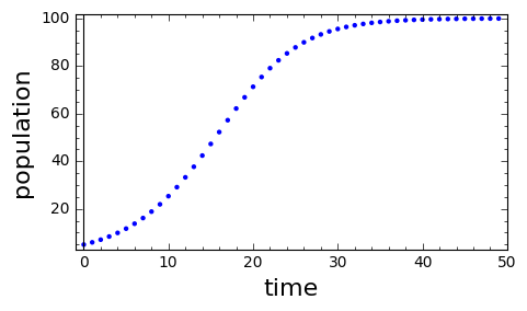
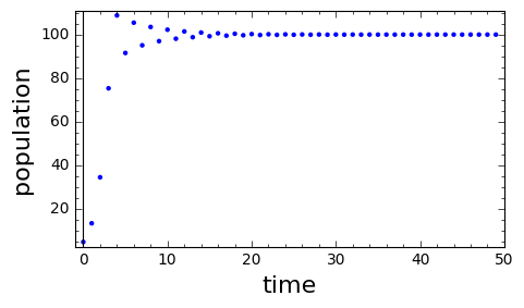
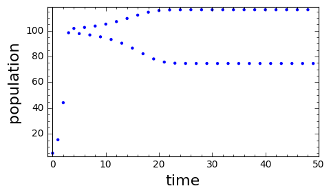
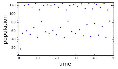
\begin{equation*} P_{t+1} = P_t + r_0\big(1-\frac{P_t}{K}\big) P_t = (1+r_0) P_t - \frac{r_0}{K} P_t^2. \end{equation*}

This model is called the discrete logistic model. The model only makes sense when the parameter $r_0$ is in the interval $r_0 \in (0,3)\text{.}$

Different behaviors for the population arise, depending on the values of the parameter $r_0\text{.}$ A Sage script is provided below that will generate plots of the population sequence for values of the parameters that you specify. The following graphs were generated by Sage using an initial value $P_0=5$ and parameter values $K=100$ (all plots) and $r_0 = 0.2\text{,}$ $r_0=1.8\text{,}$ $r_0=2.2$ and $r_0=2.6\text{.}$ In addition, a dynamic graph is given where you can adjust the parameters using sliders.

Figure 13.4.9. Dynamic graph of the discrete logistic model with variable $r$ and $P_0\text{.}$

Subsection 13.4.4 Summary

Sequences can be used to model any quantities that are observed at regular intervals, with populations and financial balances as typical examples.
A common strategy for building a recurrence model is to add rates of gain and subtract rates of loss,

\begin{equation*} \Delta x_{t} = x_{t+1}-x_t = +\text{Gains} - \text{Losses}\text{.} \end{equation*}
For a population, common gain rates include births and immigration; common loss rates include deaths and emigration.
A per capita rate is the ratio of the total rate to the population size. It represents the contribution toward the total rate for one individual. The total rate equals the per capita rate times the population size.
Finding models for individual rates or per capita rates in terms of the population size allows us to formulate a recursive equation for the population sequence. Simple examples are to assume constant rates or constant per capita rates. More complex models might fit models for density-dependent per capita rates.
We use computers to find values numerically for a sequence based on the recursive equation. This might be through a spreadsheet or through a scripting language like Python. These data allow us to create graphs.

Exercises 13.4.5 Exercises

1.

A population of annual plants has all plants die every year. Before dying, each plant releases 20 seeds which will grow the following year.

Find a recurrence equation for the population.
If $P_0=10\text{,}$ find $P_1$ and $P_2$ by hand.
Find an explicit formula for the sequence $P_t\text{.}$

2.

A population has constant per capita birth and death rates. When the population is $P=1000\text{,}$ there are $B=200$ births per year and $D=250$ deaths per year. In addition, this population has a constant immigration rate of $I=300$ individuals per year.

Find a recurrence equation for the population.
If $P_0=1000\text{,}$ find $P_1$ and $P_2$ by hand.
Use a computer to generate a plot of the sequence $(t,P_t)$ for $t=0,\ldots,50\text{.}$

3.

You put $500 in a bank which pays 1% interest, compounded annually.

Find a recurrence equation for the balance $B$ of your account. What is the initial value, $B_0\text{?}$
Compute $B_1$ and $B_2$ by hand.
Find an explicit formula for the sequence $B_t\text{.}$

4.

You inherit $50,000, which you immediately invest. Your investment fund guarantees an annual interest payment of 2%, compounded annually. You withdraw $2,000 each year to spend.

Find a recurrence equation for the balance of your fund $F\text{.}$ What is the initial value, $F_0\text{?}$
Compute $F_1$ and $F_2$ by hand.
Use a computer to generate a table and a plot of the sequence $(t,F_t)$ for $t=0,\ldots,40\text{.}$
How long will the fund last? What was the total value of the inheritance?

5.

You purchase a house with a home loan of $350,000 with an annual interest rate of 4%, which accrues monthly. You choose to make a monthly payment of $1,500.

Find a recurrence equation for the balance of your loan $L\text{.}$ What is the initial value, $L_0\text{?}$
Compute $L_1$ and $L_2$ by hand.
Use a computer to generate a table and a plot of the sequence $(t,L_t)$ for a long enough period to determine when the loan is completely paid.
When will you pay off the house loan? What will have been your total cost? How much interest will you have paid?
If you increase the monthly payments to $1,600, when will you pay off the loan? How much interest will you have paid?

6.

A pond with 100,000 gallons of water has a stream flowing in and out at a rate of 5,000 gallons per day. One day, the stream flowing in is polluted with a chemical of 200 grams per gallon. Assuming that the pond mixes the water quickly, develop a model for the amount of chemical in the pond as a daily sequence.

State your variables.
What is your model for how much chemical enters the pond each day?
What is your model for how much chemical leaves the pond each day?
State your recurrence relation and the initial value for your sequence. Determine the resulting recursive equation.
Find an explicit formula for your sequence. How much chemical is in the pond after 30 days?